
Periodic poisson problem in FEniCSx
Solving the Poisson Problem with Periodic Boundary Conditions in FEniCSx. For this we use the MultiPointConstraint library, which is built on top of FEniCSx.
In this example, we solve the Poisson problem on a 2D unit square mesh using periodic boundary conditions in the x-direction and homogeneous Dirichlet conditions in the y-direction.
We encode the periodicity in the definition of the domain:
\[\Omega = \mathbb{R}/\mathbb{Z} \times (0,1)\subset\mathbb{R}^2. \]
Given \(f:\Omega\to \mathbb{R}\), defined by
\[f(x, y) = x \sin(5\pi y) + \exp\left(-\frac{(x - 0.9)^2 + (y - 0.5)^2}{0.02}\right)\]we seek the solution \(u\in H^1_0(\Omega)\) such that
\[-\Delta u = f,\]in the weak sense.
FEniCSx is still under development, and new versions are often not 100% backwards compatible. The following code was developed for dolfinx version 0.9.0. This can be checked using
python3 -c "import dolfinx; print(dolfinx.__version__)"
or in a python file
import dolfinx
print(dolfinx.__version__)
We import the necessary modules:
from mpi4py import MPI
from petsc4py import PETSc
import dolfinx.fem as fem
import pyvista
from dolfinx import plot
import numpy as np
from dolfinx import default_scalar_type
from dolfinx.mesh import create_unit_square, locate_entities_boundary
from ufl import (
    SpatialCoordinate,
    TestFunction,
    TrialFunction,
    dx,
    exp,
    grad,
    inner,
    pi,
    sin,
)
from dolfinx_mpc import LinearProblem, MultiPointConstraint
Next, we define the mesh
# Mesh resolution
NX = 50
NY = 100
# Create unit square mesh
mesh = create_unit_square(MPI.COMM_WORLD, NX, NY)

# Define function space (Lagrange, degree 1)
V = fem.functionspace(mesh, ("Lagrange", 1))
Now we define the Dricihlet boundary conditions at \(y=0\) and \(y=1\), i.e. on the left and right of the square. The code is standard.
# Tolerance for coordinate comparisons
tol = 250 * np.finfo(default_scalar_type).resolution

# Identify top/bottom boundary (Dirichlet BC)
def dirichletboundary(x):
    return np.logical_or(np.isclose(x[1], 0, atol=tol),
                         np.isclose(x[1], 1, atol=tol))

# Apply Dirichlet BCs
facets = locate_entities_boundary(mesh, 1, dirichletboundary)
topological_dofs = fem.locate_dofs_topological(V, 1, facets)
bc = fem.dirichletbc(0., topological_dofs, V)
bcs = [bc]
We want periodic boundary conditions at \(x=0\) and \(x=1\). This is done in three steps:
- Find the relevant part of the domain (here we choose \(x=1\))
- Define the “multipoint constraint”, i.e. define happens at that part of the boundary. In our case, we want that all points with \(x=1\) should be identified with \(x=0\)
- Define the
MultiPointConstraintobject, which contains the above information and will be used in the assembly process.
# Define periodic boundary and mapping
def periodic_boundary(x):
    return np.isclose(x[0], 1, atol=tol)

def periodic_relation(x):
    out_x = np.zeros_like(x)
    out_x[0] = 1 - x[0]
    out_x[1] = x[1]
    out_x[2] = x[2]
    return out_x

# Set up periodic constraint
mpc = MultiPointConstraint(V)
mpc.create_periodic_constraint_geometrical(V, periodic_boundary, periodic_relation, bcs)
mpc.finalize()
The rest is standard again, with the only difference, that we use the LinearProblem command from the MPC library, which accepts the mpc as an argument.
# Define variational problem
u = TrialFunction(V)
v = TestFunction(V)
a = inner(grad(u), grad(v)) * dx

# Define right-hand side/source term
x = SpatialCoordinate(mesh)
dx_ = x[0] - 0.9
dy_ = x[1] - 0.5
f = x[0] * sin(5.0 * pi * x[1]) + exp(-(dx_ * dx_ + dy_ * dy_) / 0.02)
rhs = inner(f, v) * dx

# Solve the linear system
petsc_options={"ksp_type": "preonly", "pc_type": "lu"}
problem = LinearProblem(a, rhs, mpc, bcs=bcs, petsc_options=petsc_options)
uh = problem.solve()
In the following we plot the solution.
# Visualization using PyVista
cells, types, x = plot.vtk_mesh(V)
grid = pyvista.UnstructuredGrid(cells, types, x)
grid.point_data["u"] = uh.x.array.real
grid.set_active_scalars("u")
plotter = pyvista.Plotter()
warped = grid.warp_by_scalar(factor=20)
plotter.add_mesh(warped)
plotter.add_mesh(grid, show_edges=True)
plotter.show_axes()
plotter.camera_position = [(2.0, 2.0, 1.5), (0.5, 0.5, 0), (0, 0, 1)]
plotter.save_graphic("poisson_periodic_scalar.pdf")
plotter.show()
The code produces the following image:
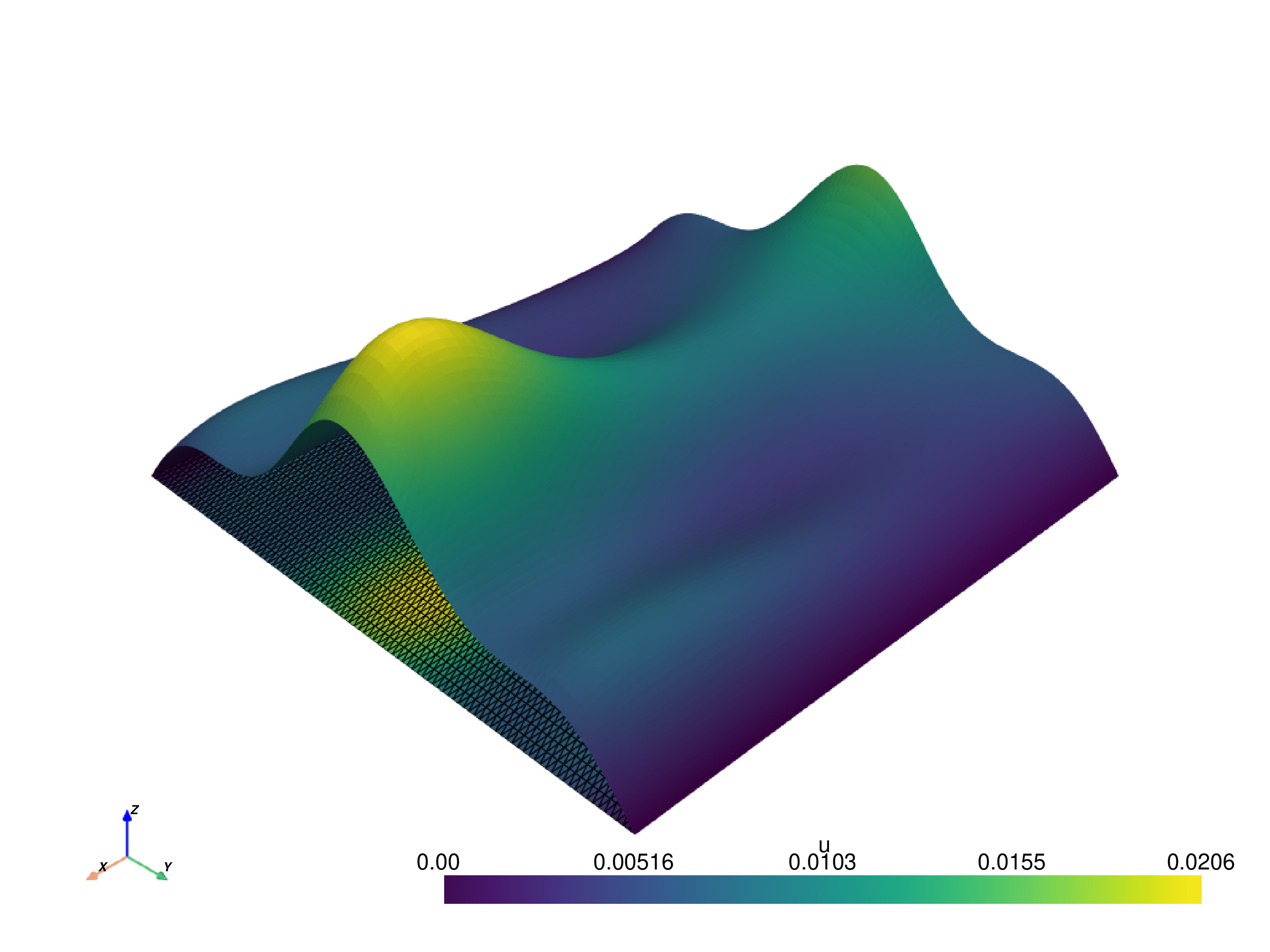
The .py file can be downloaded here.